Machine learning classification problems
Generally 2D space with various groups of samples
- 2D space with three groups of samples.
- Half moon distribution - 2D space with two variables
- ML - Regression problem
2D space with three groups of samples.
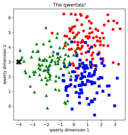
In a two-dimension space we have three groups of samples shown in the following image.
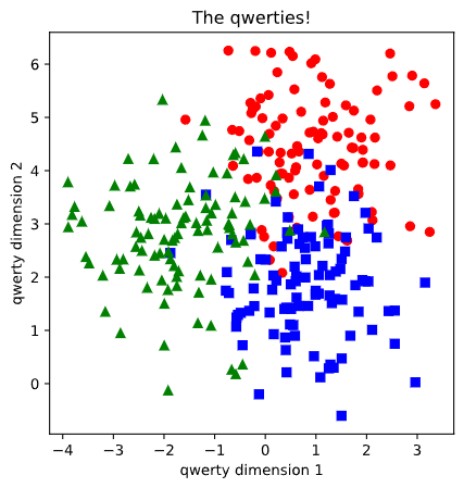
I will create a ML model that can predict to which group will belong to, a set of coordinates. In other words, can the model predict that
(-2,3) coordinate will correspond to group green. The data is called qwerties for lack of imagination.
Let’s import the modules required in python. I will use PyTorch for ML computation.
import numpy as np
import matplotlib.pyplot as plt
from sklearn.datasets import make_blobs
import matplotlib_inline
matplotlib_inline.backend_inline.set_matplotlib_formats('svg')
import torch
import torch.nn as nn
I will give myself 300 qwerties, 100 for each group red, green and blue. I create some tensors and label the colours as 0, 1 and 2. The plot is shown at the beginning.
nrPoints = 300
X, y = make_blobs(nrPoints, centers=3, n_features=2, random_state=0)
x_red = X[np.where(y==0)[0],[0]]
y_red = X[np.where(y==0)[0],[1]]
x_blue = X[np.where(y==1)[0],[1]]
y_blue = X[np.where(y==1)[0],[0]]
x_green = X[np.where(y==2)[0],[0]]
y_green = X[np.where(y==2)[0],[1]]
data = torch.tensor(X).float()
labels = torch.tensor(y).long()
fig = plt.figure(figsize=(5,5))
plt.plot(x_red, y_red,'ro')
plt.plot(x_blue, y_blue, 'bs')
plt.plot(x_green, y_green,'g^')
plt.title('The qwerties!')
plt.xlabel('qwerty dimension 1')
plt.ylabel('qwerty dimension 2')
plt.show()
Here comes the model (artificial neural network).
It has 2 inputs, 3 outputs and 4 hidden layers in between.
#model architecture
ANNq = nn.Sequential(
    nn.Linear(2,4),
    nn.ReLU(),
    nn.Linear(4,3),
    nn.Softmax(dim=1)
)

#loss function
lossfunc = nn.CrossEntropyLoss()

#optimizer
optimizer = torch.optim.Rprop(ANNq.parameters(), lr=0.1)
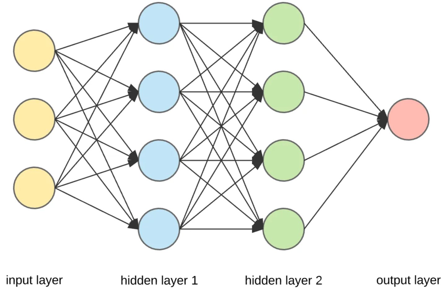
A graphical representation of ANN with 3 inputs, one output and 2 hidden layers.
The fun part begins when we need to train the model using the following code. Here I programmed the model to educate himself for 500 times, record the losses and calculate the accuracy.
#Train model
numepochs = 500

#Initial losses
losses = torch.zeros(numepochs)
ongoingAcc = []

for epochi in range(numepochs):

    #forward pass
    yHat = ANNq(data)

    #compute loss
    loss = lossfunc(yHat,labels)
    losses[epochi] = loss

    #backprop
    optimizer.zero_grad()
    loss.backward()
    optimizer.step()

    #compute accuracy
    matches = torch.argmax(yHat,axis=1) == labels   #boolean false or true
    matchesNumeric = matches.float()                #convert to 0/1
    accuracyPct = 100 * torch.mean(matchesNumeric)  #acerage and *100
    ongoingAcc.append( accuracyPct )                # add to the list of accuracy


#final forward pass
predictions = ANNq(data)

predlabels = torch.argmax(predictions,axis=1)
totalacc = 100 * torch.mean((predlabels == labels).float())
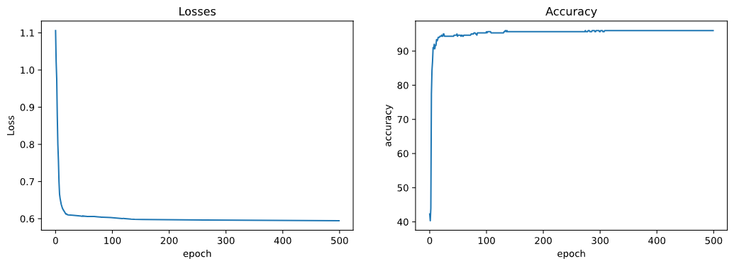
Best way is to visualize the losses and accuracy. It seems to be a fast learner. He could’ve finish his self education after only 100 trials.
Another smart way to show some outcome of the model is to plot the probability of each group. One colour will have 100 probability and the other two will have 0.
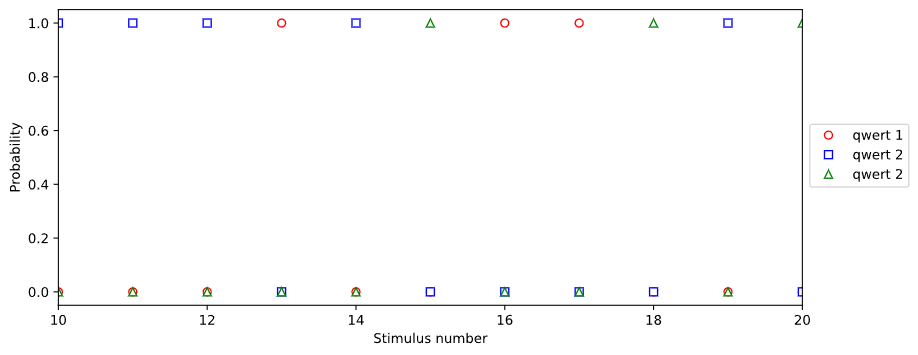
We can save the trained model and later utilize the already trained model which is much faster. Complicated models can take hours or days to train.
#Save model
torch.save(ANNq.state_dict(),'traniedModel.pt')

#Another user can load the model
#Load the pre-trained model
loaded_model = ANNq
loaded_model.load_state_dict(torch.load('traniedModel.pt'))
loaded_model.eval()
Let’s test the trained model:
#Testing the model
X_test = [[np.random.randint(-4,4), np.random.randint(-1,6)]]
test_data = torch.tensor(X_test).float()
results = loaded_model(test_data)
print('test numers: ', X_test)
print(results.detach())
if results[0,0].detach() == 1 :
    print('red')
elif results[0,1].detach() == 1 :
    print('blue')
else:
    print('green')
Here is the output:
test numbers: [[-4, 3]]
tensor([[2.7208e-40, 0.0000e+00, 1.0000e+00]])
The coordinate correspond to group: green
And the final result:
Half moon distribution - 2D space with two variables
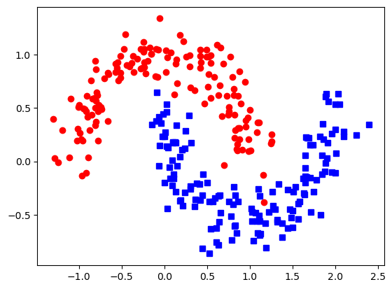
If we have a preferential distribution it is somehow more difficult to predict the classifications using conventional statistical approach.
Here is the plot with two input values and two preferential distributed zones :
We import the python modules:
from sklearn.datasets import make_moons
import matplotlib.pyplot as plt
import numpy as np
import torch as tch
import torch.nn as nn
X, y = make_moons(n_samples=300, noise=0.15, random_state=0)
data = tch.tensor(X).float()
labels = tch.tensor(y).long()
plt.plot(data[labels==0,0], data[labels==0,1],'ro')
plt.plot(data[labels==1,0], data[labels==1,1], 'bs')
plt.show()
My approach for ANN model is to use 4 hidden layers:
#create the model layout

model = nn.Sequential(
    nn.Linear(2,4),   #input layer
    nn.ReLU(),        #activation layer
    nn.Linear(4,2),   #Output layer
    nn.Softmax(dim=1)
)

# loss function
lossfun = nn.CrossEntropyLoss()

#optimizer
optimizer = tch.optim.SGD(model.parameters(),lr=0.05)
The code to train the model going through 10000 trials:
#train the model
numepoch = 10000
losses = tch.zeros(numepoch)


for epochi in range(numepoch):
    #forward pass
    yHat = model(data)

    #compute losses
    loss = lossfun(yHat,labels)
    losses[epochi] = loss

    #backpropagation
    optimizer.zero_grad()
    loss.backward()
    optimizer.step()

#final forward pass
predictions = model(data)

#compute prediction accuracy
predlabels = tch.argmax(predictions,axis=1)
totalacc = 100 * tch.mean((predlabels == labels).float())

# report accuracy
print('Final accuracy: %g%%' %totalacc)

plt.plot(losses.detach())
plt.show()
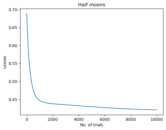
Final accuracy is 87.6 %. The model struggle a bit in the beginning according with losses plot.
We switch the model into evaluation mode from training mode and test with the coordinates [1,1] and hope it will predict red:
  model.eval()
  X_test = [[1, 1]]
test_data = tch.tensor(X_test).float()
results = model(test_data)
label_results = tch.argmax(results,axis=1)

print('test numers: ', X_test)
print(label_results)

if label_results.detach() == 0 :
    print('red')
else:
    print('blue')
test numers:  [[1, 1]]
tensor([0])
red
Indeed.
ML - Regression problem
A simple regression example - 2D space y = ax + b.
This is a simple 2D regression as it help visualize the problem and the solution. This will be suitable for multiple inputs and outputs which is difficult to visualize in our limited 3D space.
The equation will be y = -5 * x +0.1 * random numbers between -5 and 5.
import torch
import matplotlib.pyplot as plt


#Data input
x = torch.arange(-5, 5, 0.1).view(-1, 1)
y = -5 * x + 0.1 * torch.randn(x.size())


#Define the model backbone
model = torch.nn.Linear(1, 1)                               #Model type - Linear
criterion = torch.nn.MSELoss()                              #measure the losses - Mean Squared Error between iput and target
optimizer = torch.optim.SGD(model.parameters(), lr = 0.1)   #Stochastic gradient desent - derivative to find the minimum
The function to train the model:
def train_model(iter):
    for epoch in range(iter):
        y1 = model(x)                                        #Put x into the model
        loss = criterion(y1, y)                              #Calculates the loss
        optimizer.zero_grad()                                #Finds the minimum
        loss.backward()                                      #Computes the dloss/dx
        optimizer.step()                                     #Updates the value of x using gradient optimizer.zero_grad

net = train_model(10)                                        # 10 iterations are enough to get the regression
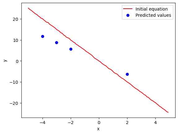
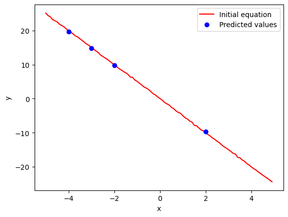
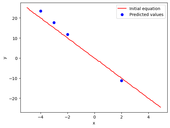
Let’s test the model for -4, -3, -2 and 2 plot against the linear equation.
#Test the model with one value -4
X = torch.tensor([[-4.0], [-3.0], [-2], [2]])

yhat = model(X)                 #Calculates y for x=-4 # yhat is the local minimum of a diferentiable funtion

plt.plot(x, y, 'r-')
plt.plot(X, yhat.detach(), 'bo')
plt.show()
This is the plot after 10 iterations:
And after only 5 iterations:
How about two iterations: